Electric Propulsion Basics¶

Electrostatic Thrust Generation¶

Like all rockets, electric thrusters generate thrust by expelling mass at high velocity. In electric (electrostatic) propulsion, a high-velocity jet is produced by accelerating charged particles through an electric potential.

The propellant medium in electrostatic thrusters is a plasma consisting of electrons and positively charged ions. The plasma is usually produced by ionizing a gas via electron bombardment. The electric fields within the thruster are configured such that there is a large potential drop between the plasma generation region and the thruster exit. When ions exit the thruster, the are accelerated to high velocities by the electrostatic force. If the ions fall through a beam potential of \(V_b\), they will leave the thruster with a velocity

\[v_e = \sqrt{2 V_b \frac{q}{m_i}}\]

where \(q\) is the ion charge and \(m_i\) is the ion mass. The thrust produced by the ion flow is

\[ \begin{align}\begin{aligned}F &= v_e \dot{m}\\ &= \left( \sqrt{2 V_b \frac{q}{m_i}} \right) \left( \frac{m_i}{q} I_b \right)\\ &= I_b \sqrt{2 V_b \frac{m_i}{q}}\end{aligned}\end{align} \]

where \(I_b\) is the ion beam current.

The ideal specific impulse of an electrostatic thruster is:

\[ \begin{align}\begin{aligned}I_{sp} &= \frac{v_e}{g_0}\\ &= \frac{1}{g_0} \sqrt{2 V_b \frac{q}{m_i}}\end{aligned}\end{align} \]

As an example, use proptools to compute the thrust and specific impulse of singly charged Xenon ions with a beam voltage of 1000 V and a beam current of 1 A:

"""Example electric propulsion thrust and specific impulse calculation."""
from proptools import electric, constants

V_b = 1000.    # Beam voltage [units: volt].
I_b = 1.    # Beam current [units: ampere].
F = electric.thrust(I_b, V_b, electric.m_Xe)
I_sp = electric.specific_impulse(V_b, electric.m_Xe)
m_dot = F / (I_sp * constants.g)
print 'Thrust = {:.1f} mN'.format(F * 1e3)
print 'Specific Impulse = {:.0f} s'.format(I_sp)
print 'Mass flow = {:.2f} mg s^-1'.format(m_dot * 1e6)

Thrust = 52.2 mN

Specific Impulse = 3336 s

Mass flow = 1.59 mg s^-1

This example illustrates the typical performance of electric propulsion systems: low thrust, high specific impulse, and low mass flow.

Advantages over Chemical Propulsion¶

Electric propulsion is appealing because it enables higher specific impulse than chemical propulsion. The specific impulse of a chemical rocket depends on velocity to which a nozzle flow can be accelerated. This velocity is limited by the finite energy content of the working gas. In contrast, the particles leaving an electric thruster can be accelerated to very high velocities if sufficient electrical power is available.

In a chemical rocket, the kinetic energy of the exhaust gas is supplied by thermal energy released in a combustion reaction. For example, in the stoichiometric combustion of H₂ and O₂ releases an energy per particle of \(4.01 \times 10^{-19}\) J, or 2.5 eV. If all of the released energy were converted into kinetic energy of the exhaust jet, the maximum possible exhaust velocity would be:

\[v_e = \sqrt{2 \frac{E}{m_{H_2O}}} = 5175 \, \mathrm{m s^{-1}}\]

corresponding to a maximum specific impulse of about 530 s. In practice, the most efficient flight engines have specific impulses of 450 to 500 s.

With electric propulsion, much higher energies per particle are possible. If we accelerate (singly) charged particles through a potential of 1000 V, the jet kinetic energy will be 1000 eV per ion. This is 400 times more energy per particle than is possible with chemical propulsion (or, for similar particle masses, 20 times higher specific impulse). Specific impulse in excess of 10,000 s is feasible with electric propulsion.

Power and Efficiency¶

In an electric thruster, the energy to accelerate the particles in the jet must be supplied by an external source. Typically solar panels supply this electrical power, but some future concepts might use nuclear reactors. The available power limits the thrust and specific impulse of an electric thruster.

The kinetic power of the jet is given by:

\[P_{jet} = \frac{F^2}{2 \dot{m}}\]

where \(\dot{m}\) is the jet mass flow. Increasing thrust with increasing mass flow (i.e. increasing \(I_{sp}\)) will increase the kinetic power of the jet.

The power input required by the thruster (\(P_{in}\)) is somewhat higher than the jet power. The ratio of the jet and input power is the total efficiency of the thruster, \(\eta_T\):

\[\eta_T \equiv \frac{P_{jet}}{P_{in}}\]

The total efficiency depends on several factors:

Thrust losses due to beam divergence. This loss is proportional to the cosine of the average beam divergence half-angle.
Thrust losses due to doubly charged ions in the beam. This loss is a function of the doubles-to-singles current ratio, \(I^{++}/I^+\)
Thrust losses due to propellant gas escaping the thruster without being ionized. The fraction of the propellant mass flow which is ionized and enters the beam is the mass utilization efficiency, \(\eta_m\).
Electrical losses incurred in ion generation, power conversion, and powering auxiliary thruster components. These losses are captured by the electrical efficiency, \(\eta_e = \frac{I_b V_b}{P_{in}}\)

Use proptools to compute the efficiency and required power of the example thruster. Assume that the beam divergence is \(\cos(10 \unicode{xb0})\), the double ion current fraction is 10%, the mass utilization efficiency is 90%, and the electrical efficiency is 85%:

"""Example electric propulsion power calculation."""
import numpy as np
from proptools import electric

F = 52.2e-3    # Thrust [units: newton].
m_dot = 1.59e-6    # Mass flow [units: kilogram second**-1].

# Compute the jet power [units: watt].
P_jet = electric.jet_power(F, m_dot)

# Compute the total efficiency [units: dimensionless].
eta_T = electric.total_efficiency(
    divergence_correction=np.cos(np.deg2rad(10)),
    double_fraction=0.1,
    mass_utilization=0.9,
    electrical_efficiency=0.85)

# Compute the input power [units: watt].
P_in = P_jet / eta_T

print 'Jet power = {:.0f} W'.format(P_jet)
print 'Total efficiency = {:.3f}'.format(eta_T)
print 'Input power = {:.0f} W'.format(P_in)

Jet power = 857 W

Total efficiency = 0.703

Input power = 1219 W

The overall efficiency of the thruster is about 70%. The required input power could be supplied by a few square meters of solar panels (at 1 AU from the sun).

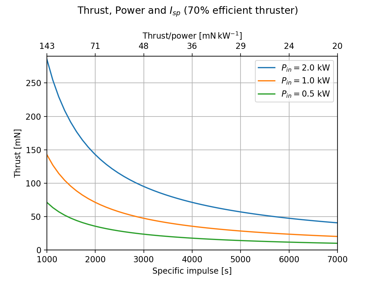
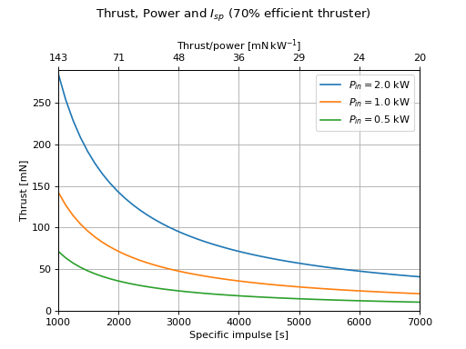
The power, thrust, and specific impulse of a thruster are related by:

\[\frac{F}{P_{in}} = \frac{2 \eta_T}{g_0 I_{sp}}\]

Thus, for a power-constrained system the propulsion designer faces a trade-off between thrust and specific impulse.

"""Plot the thrust, power, Isp trade-off."""
from matplotlib import pyplot as plt
import numpy as np
from proptools import electric

eta_T = 0.7    # Total efficiency [units: dimensionless].
I_sp = np.linspace(1e3, 7e3)    # Specific impulse [units: second].

ax1 = plt.subplot(111)
for P_in in [2e3, 1e3, 500]:
    T = P_in * electric.thrust_per_power(I_sp, eta_T)
    plt.plot(I_sp, T * 1e3, label='$P_{{in}} = {:.1f}$ kW'.format(P_in * 1e-3))

plt.xlim([1e3, 7e3])
plt.ylim([0, 290])
plt.xlabel('Specific impulse [s]')
plt.ylabel('Thrust [mN]')
plt.legend()
plt.suptitle('Thrust, Power and $I_{sp}$ (70% efficient thruster)')
plt.grid(True)

# Add thrust/power on second axis.
ax2 = ax1.twiny()
new_tick_locations = ax1.get_xticks()
ax2.set_xlim(ax1.get_xlim())
ax2.set_xticks(new_tick_locations)
ax2.set_xticklabels(['{:.0f}'.format(tp * 1e6)
                     for tp in electric.thrust_per_power(new_tick_locations, eta_T)])
ax2.set_xlabel('Thrust/power [$\\mathrm{mN \\, kW^{-1}}$]')
ax2.tick_params(axis='y', direction='in', pad=-25)
plt.subplots_adjust(top=0.8)

plt.show()

(Source code, png, hires.png, pdf)

Optimal Specific Impulse¶

For electrically propelled spacecraft, there is an optimal specific impulse which will maximize the payload mass fraction of a given mission. While increasing specific impulse decreases the required propellant mass, it also increases the required power at a particular thrust level, which increases the mass of the power supply. The optimal specific impulse minimizes the combined mass of the propellant and power supply.

The optimal specific impulse depends on several factors:

The mission thrust duration, \(t_m\). Longer thrust durations reduce the required thrust (if the same total impulse or \(\Delta v\) is to be delivered), and therefore reduce the power and power supply mass at a given \(I_{sp}\). Therefore, longer thrust durations increase the optimal \(I_{sp}\).
The specific mass of the power supply, \(\alpha\). This is the ratio of power supply mass to power, and is typically 20 to 200 kg kW ^-1 for solar-electric systems. The specific impulse optimization assumes that power supply mass is linear with respect to power. Increasing the specific mass reduces the optimal \(I_{sp}\).
The total efficiency of the thruster.
The \(\Delta v\) of the mission. Higher \(\Delta v\) (in a fixed time window) requires more thrust, and therefore leads to a lower optimal \(I_{sp}\).

Consider an example mission to circularize the orbit of a geostationary satellite launched onto a elliptical transfer orbit. Assume that the low-thrust circularization maneuver requires a \(\Delta v\) of 2 km s ^-1 over 100 days. The thruster is 70% efficient and the power supply specific mass is 50 kg kW ^-1:

"""Example calculation of optimal specific impulse for an electrically propelled spacecraft."""
from proptools import electric

dv = 2e3    # Delta-v [units: meter second**-1].
t_m = 100 * 24 * 60 * 60    # Thrust duration [units: second].
eta_T = 0.7    # Total efficiency [units: dimensionless].
specific_mass = 50e-3    # Specific mass of poower supply [units: kilogram watt**-1].
I_sp = electric.optimal_isp_delta_v(dv, eta_T, t_m, specific_mass)

print 'Optimal specific impulse = {:.0f} s'.format(I_sp)

Optimal specific impulse = 1482 s

For the mathematical details of specific impulse optimization, see [Lozano].

[Lozano]

Lozano, 16.522 Lecture Notes, Lecture 3-4 Mission Analysis for Electric Propulsion. Online: https://ocw.mit.edu/courses/aeronautics-and-astronautics/16-522-space-propulsion-spring-2015/lecture-notes/MIT16_522S15_Lecture3-4.pdf