Nozzle Flow
Nozzle flow theory can predict the thrust and specific impulse of a rocket engine. The following example predicts the performance of an engine which operates at chamber pressure of 10 MPa, chamber temperature of 3000 K, and has 100 mm diameter nozzle throat.
"""Estimate specific impulse, thrust and mass flow."""
from math import pi
from proptools import nozzle

# Declare engine design parameters
p_c = 10e6    # Chamber pressure [units: pascal]
p_e = 100e3    # Exit pressure [units: pascal]
gamma = 1.2    # Exhaust heat capacity ratio [units: dimensionless]
m_molar = 20e-3    # Exhaust molar mass [units: kilogram mole**1]
T_c = 3000.    # Chamber temperature [units: kelvin]
A_t = pi * (0.1 / 2)**2    # Throat area [units: meter**2]

# Predict engine performance
C_f = nozzle.thrust_coef(p_c, p_e, gamma)    # Thrust coefficient [units: dimensionless]
c_star = nozzle.c_star(gamma, m_molar, T_c)    # Characteristic velocity [units: meter second**-1]
I_sp = C_f * c_star / nozzle.g    # Specific impulse [units: second]
F = A_t * p_c * C_f    # Thrust [units: newton]
m_dot = A_t * p_c / c_star    # Propellant mass flow [units: kilogram second**-1]

print 'Specific impulse = {:.1f} s'.format(I_sp)
print 'Thrust = {:.1f} kN'.format(F * 1e-3)
print 'Mass flow = {:.1f} kg s**-1'.format(m_dot)
Output:
Specific impulse = 288.7 s

Thrust = 129.2 kN

Mass flow = 45.6 kg s**-1
The rest of this page derives the nozzle flow theory, and demonstrates other features of proptools.nozzle.
Ideal Nozzle Flow
The purpose of a rocket is to generate thrust by expelling mass at high velocity. The rocket nozzle is a flow device which accelerates gas to high velocity before it is expelled from the vehicle. The nozzle accelerates the gas by converting some of the gas’s thermal energy into kinetic energy.
Ideal nozzle flow is a simplified model of the aero- and thermo-dynamic behavior of fluid in a nozzle. The ideal model allows us to write algebraic relations between an engine’s geometry and operating conditions (e.g. throat area, chamber pressure, chamber temperature) and its performance (e.g. thrust and specific impulse). These equations are fundamental tools for the preliminary design of rocket propulsion systems.
The assumptions of the ideal model are:
- The fluid flowing through the nozzle is gaseous.
- The gas is homogeneous, obeys the ideal gas law, and is calorically perfect. Its molar mass (\(\mathcal{M}\)) and heat capacities (\(c_p, c_v\)) are constant throughout the fluid, and do not vary with temperature.
- There is no heat transfer to or from the gas. Therefore, the flow is adiabatic. The specific enthalpy \(h\) is constant throughout the nozzle.
- There are no viscous effects or shocks within the gas or at its boundaries. Therefore, the flow is reversible. If the flow is both adiabatic and reversible, it is isentropic: the specific entropy \(s\) is constant throughout the nozzle.
- The flow is steady; \(\frac{d}{dt} = 0\).
- The flow is quasi one dimensional. The flow state varies only in the axial direction of the nozzle.
- The flow velocity is axially directed.
- The flow does not react in the nozzle. The chemical equilibrium established in the combustion chamber does not change as the gas flows through the nozzle. This assumption is known as “frozen flow”.
These assumptions are usually acceptably accurate for preliminary design work. Most rocket engines perform within 1% to 6% of the ideal model predictions [RPE].
Isentropic Relations
Under the assumption of isentropic flow and calorically perfect gas, there are several useful relations between fluid states. These relations depend on the heat capacity ratio, \(\gamma = c_p /c_v\). Consider two gas states, 1 and 2, which are isentropically related (\(s_1 = s_2\)). The states’ pressure, temperature and density ratios are related:
Stagnation state
Now consider the relation between static and stagnation states in a moving fluid. The stagnation state is the state a moving fluid would reach if it were isentropically decelerated to zero velocity. The stagnation enthalpy \(h_0\) is the sum of the static enthalpy and the specific kinetic energy:
For a calorically perfect gas, \(T = h / c_p\), and the stagnation temperature is:
It is helpful to write the fluid properties in terms of the Mach number \(M\), instead of the velocity. Mach number is the velocity normalized by the local speed of sound, \(a = \sqrt{\gamma R T}\). In terms of Mach number, the stagnation temperature is:
Because the static and stagnation states are isentropically related, \(\frac{p_0}{p} = \left( \frac{T_0}{T} \right)^{\frac{\gamma}{\gamma - 1}}\). Therefore, the stagnation pressure is:
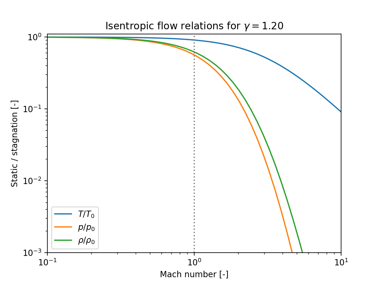
Use proptools to plot the stagnation state variables against Mach number:
"""Plot isentropic relations."""
import numpy as np
from matplotlib import pyplot as plt
from proptools import isentropic

M = np.logspace(-1, 1)
gamma = 1.2

plt.loglog(M, 1 / isentropic.stag_temperature_ratio(M, gamma), label='$T / T_0$')
plt.loglog(M, 1 / isentropic.stag_pressure_ratio(M, gamma), label='$p / p_0$')
plt.loglog(M, 1 / isentropic.stag_density_ratio(M, gamma), label='$\\rho / \\rho_0$')
plt.xlabel('Mach number [-]')
plt.ylabel('Static / stagnation [-]')
plt.title('Isentropic flow relations for $\gamma={:.2f}$'.format(gamma))
plt.xlim(0.1, 10)
plt.ylim([1e-3, 1.1])
plt.axvline(x=1, color='grey', linestyle=':')
plt.legend(loc='lower left')
plt.show()
(Source code, png, hires.png, pdf)
Exit velocity
The exit velocity of the exhaust gas is the fundamental measure of efficiency for rocket propulsion systems, as the rocket equation shows. We can now show a basic relation between the exit velocity and the combustion conditions of the rocket. First, use the conservation of energy to relate the velocity at any two points in the flow:
We can replace the enthalpy difference with an expression of the pressures and temperatures, using the isentropic relations.
Set state 1 to be the conditions in the combustion chamber: \(T_1 = T_c, p_1 = p_c, v_1 \approx 0\). Set state 2 to be the state at the nozzle exit: \(p_2 = p_e, v_2 = v_e\). This gives the exit velocity:
where \(\mathcal{R} = 8.314\) J mol -1 K -1 is the universal gas constant and \(\mathcal{M}\) is the molar mass of the exhaust gas. Temperature and molar mass have the most significant effect on exit velocity. To maximize exit velocity, a rocket should burn propellants which yield a high flame temperature and low molar mass exhaust. This is why many rockets burn hydrogen and oxygen: they yield a high flame temperature, and the exhaust (mostly H2 and H2O) is of low molar mass.
The pressure ratio \(p_e / p_c\) is usually quite small. As the pressure ratio goes to zero, the exit vleocity approaches its maximum for a given \(T_c, \mathcal{M}\) and \(\gamma\).
If \(p_e \ll p_c\), the pressures have a weak effect on exit velocity.
The heat capacity ratio \(\gamma\) has a weak effect on exit velocity. Decreasing \(\gamma\) increases exit velocity.
Use proptools to find the exit velocity of the example engine:
"""Estimate exit velocity."""
from proptools import isentropic

# Declare engine design parameters
p_c = 10e6    # Chamber pressure [units: pascal]
p_e = 100e3    # Exit pressure [units: pascal]
gamma = 1.2    # Exhaust heat capacity ratio [units: dimensionless]
m_molar = 20e-3    # Exhaust molar mass [units: kilogram mole**1]
T_c = 3000.    # Chamber temperature [units: kelvin]

# Compute the exit velocity
v_e = isentropic.velocity(v_1=0, p_1=p_c, T_1=T_c, p_2=p_e, gamma=gamma, m_molar=m_molar)

print 'Exit velocity = {:.0f} m s**-1'.format(v_e)
Exit velocity = 2832 m s**-1
Mach-Area Relation
Using the isentropic relations, we can find how the Mach number of the flow varies with the cross sectional area of the nozzle. This allows the design of a nozzle geometry which will accelerate the flow the high speeds needed for rocket propulsion.
Start with the conservation of mass. Because the flow is quasi- one dimensional, the mass flow through every cross-section of the nozzle must be the same:
where \(A\) is the cross-sectional area of the nozzle flow passage (normal to the flow axis). To conserve mass, the ratio of areas between any two points along the nozzle axis must be:
Use the isentropic relations to write the velocity and density in terms of Mach number, and simplify:
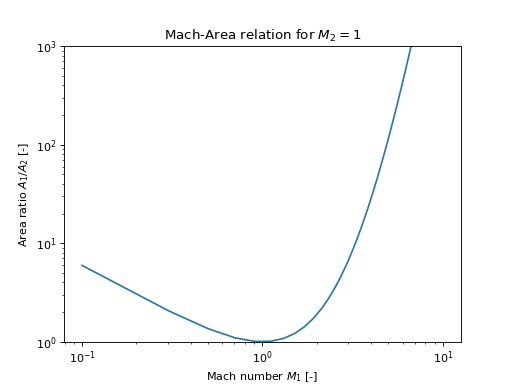
We can use proptools to plot Mach-Area relation. Let \(M_2 = 1\) and plot \(A_1 / A_2\) vs \(M_1\):
"""Plot the Mach-Area relation."""
import numpy as np
from matplotlib import pyplot as plt
from proptools import nozzle

M_1 = np.linspace(0.1, 10)    # Mach number [units: dimensionless]
gamma = 1.2    # Exhaust heat capacity ratio [units: dimensionless]

area_ratio = nozzle.area_from_mach(M_1, gamma)

plt.loglog(M_1, area_ratio)
plt.xlabel('Mach number $M_1$ [-]')
plt.ylabel('Area ratio $A_1 / A_2$ [-]')
plt.title('Mach-Area relation for $M_2 = 1$')
plt.ylim([1, 1e3])
plt.show()
(Source code, png, hires.png, pdf)

We see that the nozzle area has a minimum at \(M = 1\). At subsonic speeds, Mach number increases as the area is decreased. At supersonic speeds (\(M > 1\)), Mach number increases as area increases. For a flow passage to accelerate gas from subsonic to supersonic speeds, it must first decrease in area, then increase in area. Therefore, most rocket nozzles have a convergent-divergent shape. Larger expansions of the divergent section lead to higher exit Mach numbers.
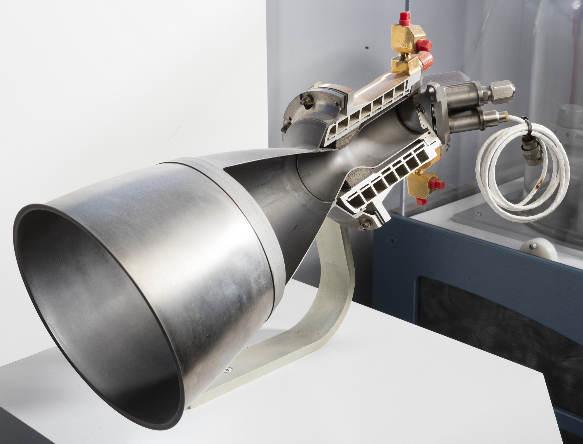
The typical converging-diverging shape of rocket nozzles is shown in this cutaway of the Thiokol C-1 engine. Image credit: Smithsonian Institution, National Air and Space Museum
Choked Flow
The station of minimum area in a converging-diverging nozzle is known as the nozzle throat. If the pressure ratio across the nozzle is at least:
then the flow at the throat will be sonic (\(M = 1\)) and the flow in the diverging section will be supersonic. The velocity at the throat is:
The mass flow at the sonic throat (i.e. through the nozzle) is:
Notice that the mass flow does not depend on the exit pressure. If the exit pressure is sufficiently low to produce sonic flow at the throat, the nozzle is choked and further decreases in exit pressure will not alter the mass flow. Increasing the chamber pressure increases the density at the throat, and therefore will increase the mass flow which can “fit through” the throat. Increasing the chamber temperature increases the throat velocity but decreases the density by a larger amount; the net effect is to decrease mass flow as \(1 / \sqrt{T_c}\).
Use proptools to compute the mass flow of the example engine:
"""Check that the nozzle is choked and find the mass flow."""
from math import pi
from proptools import nozzle

# Declare engine design parameters
p_c = 10e6    # Chamber pressure [units: pascal]
p_e = 100e3    # Exit pressure [units: pascal]
gamma = 1.2    # Exhaust heat capacity ratio [units: dimensionless]
m_molar = 20e-3    # Exhaust molar mass [units: kilogram mole**1]
T_c = 3000.    # Chamber temperature [units: kelvin]
A_t = pi * (0.1 / 2)**2    # Throat area [units: meter**2]

# Check choking
if nozzle.is_choked(p_c, p_e, gamma):
    print 'The flow is choked'

# Compute the mass flow [units: kilogram second**-1]
m_dot = nozzle.mass_flow(A_t, p_c, T_c, gamma, m_molar)

print 'Mass flow = {:.1f} kg s**-1'.format(m_dot)
The flow is choked

Mass flow = 45.6 kg s**-1
Thrust
The thrust force of a rocket engine is equal to the momentum flow out of the nozzle plus a pressure force at the nozzle exit:
where \(p_a\) is the ambient pressure and \(A_e\) is the nozzle exit area. We can rewrite this in terms of the chamber pressure:
Note that thrust depends only on \(\gamma\) and the nozzle pressures and areas; not chamber temperature.
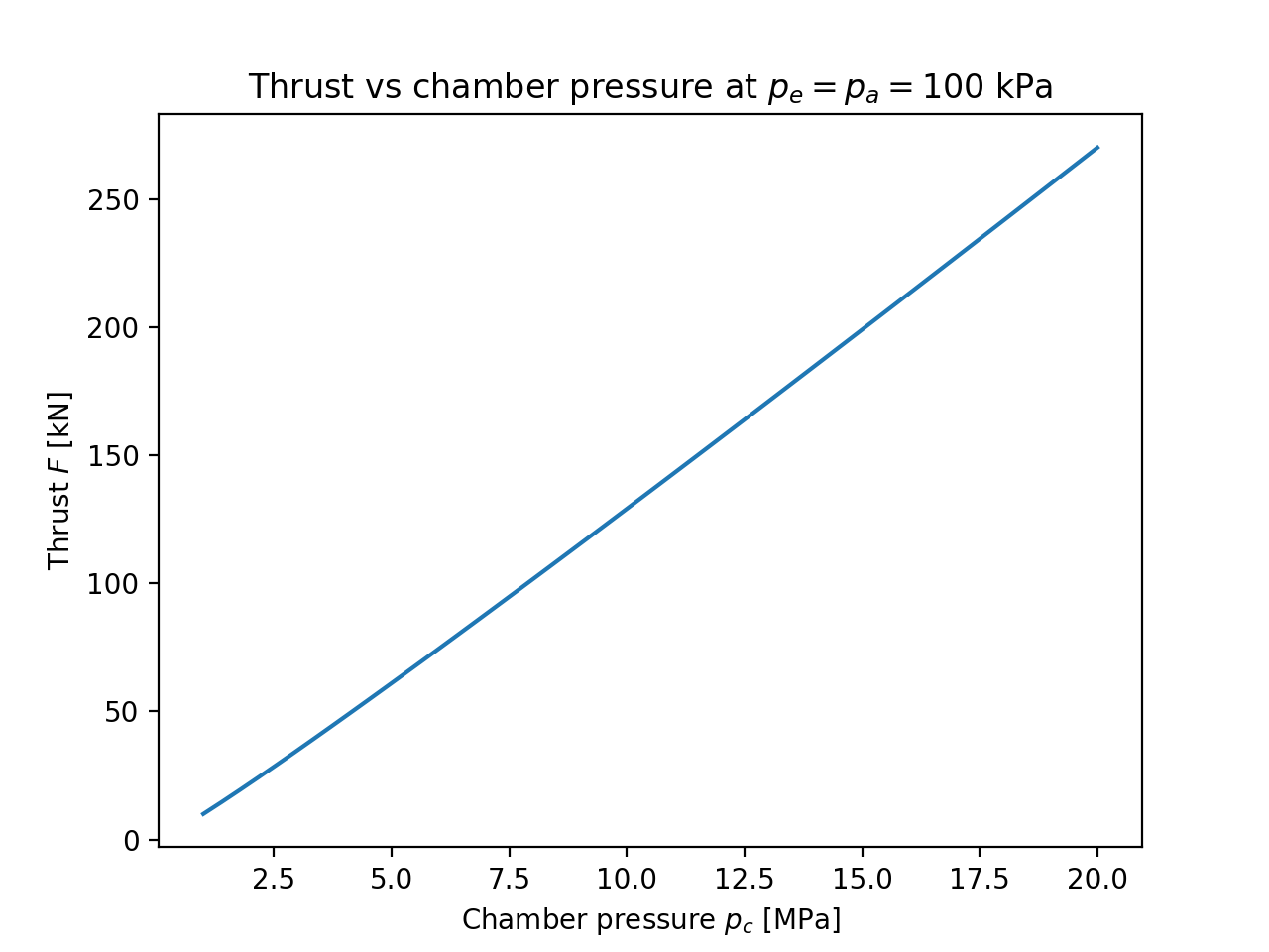
Use proptools to plot thrust versus chamber pressure for the example engine:
"""Plot thrust vs chmaber pressure."""

import numpy as np
from matplotlib import pyplot as plt
from proptools import nozzle

p_c = np.linspace(1e6, 20e6)    # Chamber pressure [units: pascal]
p_e = 100e3    # Exit pressure [units: pascal]
p_a = 100e3    # Ambient pressure [units: pascal]
gamma = 1.2    # Exhaust heat capacity ratio [units: dimensionless]
A_t = np.pi * (0.1 / 2)**2    # Throat area [units: meter**2]

# Compute thrust [units: newton]
F = nozzle.thrust(A_t, p_c, p_e, gamma)

plt.plot(p_c * 1e-6, F * 1e-3)
plt.xlabel('Chamber pressure $p_c$ [MPa]')
plt.ylabel('Thrust $F$ [kN]')
plt.title('Thrust vs chamber pressure at $p_e = p_a = {:.0f}$ kPa'.format(p_e * 1e-3))
plt.show()
(Source code, png, hires.png, pdf)
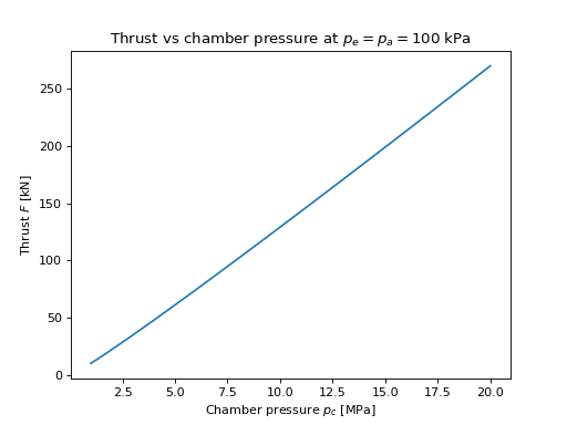
Note that thrust is almost linear in chamber pressure.
We can also explore the variation of thrust with ambient pressure for fixed \(p_c, p_e\):
"""Plot thrust vs ambient pressure."""
import numpy as np
from matplotlib import pyplot as plt
import skaero.atmosphere.coesa as atmo
from proptools import nozzle

p_c = 10e6   # Chamber pressure [units: pascal]
p_e = 100e3    # Exit pressure [units: pascal]
p_a = np.linspace(0, 100e3)    # Ambient pressure [units: pascal]
gamma = 1.2    # Exhaust heat capacity ratio [units: dimensionless]
A_t = np.pi * (0.1 / 2)**2    # Throat area [units: meter**2]

# Compute thrust [units: newton]
F = nozzle.thrust(A_t, p_c, p_e, gamma,
                  p_a=p_a, er=nozzle.er_from_p(p_c, p_e, gamma))

ax1 = plt.subplot(111)
plt.plot(p_a * 1e-3, F * 1e-3)
plt.xlabel('Ambient pressure $p_a$ [kPa]')
plt.ylabel('Thrust $F$ [kN]')
plt.suptitle('Thrust vs ambient pressure at $p_c = {:.0f}$ MPa, $p_e = {:.0f}$ kPa'.format(
    p_c *1e-6, p_e * 1e-3))

# Add altitude on second axis
ylim = plt.ylim()
ax2 = ax1.twiny()
new_tick_locations = np.array([100, 75, 50, 25, 1])
ax2.set_xlim(ax1.get_xlim())
ax2.set_xticks(new_tick_locations)


def tick_function(p):
    """Map atmospheric pressure [units: kilopascal] to altitude [units: kilometer]."""
    h_table = np.linspace(84e3, 0)    # altitude [units: meter]
    p_table = atmo.pressure(h_table)    # atmo pressure [units: pascal]
    return np.interp(p * 1e3, p_table, h_table) * 1e-3


ax2.set_xticklabels(['{:.0f}'.format(h) for h in tick_function(new_tick_locations)])
ax2.set_xlabel('Altitude [km]')
ax2.tick_params(axis='y', direction='in', pad=-25)
plt.subplots_adjust(top=0.8)
plt.show()
Thrust coefficient
We can normalize thrust by \(A_t p_c\) to give a non-dimensional measure of nozzle efficiency, which is independent of engine size or power level. This is the thrust coefficient, \(C_F\):
For an ideal nozzle, the thrust coefficient is:
Note that \(C_F\) is independent of the combustion temperature or the engine size. It depends only on the heat capacity ratio, nozzle pressures, and expansion ratio (\(A_e / A_t\)). Therefore, \(C_F\) is a figure of merit for the nozzle expansion process. It can be used to compare the efficiency of different nozzle designs on different engines. Values of \(C_F\) are generally between 0.8 and 2.2, with higher values indicating better nozzle performance.
Expansion Ratio
The expansion ratio is an important design parameter which affects nozzle efficiency. It is the ratio of exit area to throat area:
The expansion ratio appears directly in the equation for thrust coefficient. The expansion ratio also allows the nozzle designer to set the exit pressure. The relation between expansion ratio and pressure ratio can be found from mass conservation and the isentropic relations:
This relation is implemented in proptools:
"""Compute the expansion ratio for a given pressure ratio."""
from proptools import nozzle

p_c = 10e6    # Chamber pressure [units: pascal]
p_e = 100e3    # Exit pressure [units: pascal]
gamma = 1.2    # Exhaust heat capacity ratio [units: dimensionless]

# Solve for the expansion ratio [units: dimensionless]
exp_ratio = nozzle.er_from_p(p_c, p_e, gamma)

print 'Expansion ratio = {:.1f}'.format(exp_ratio)
Expansion ratio = 11.9
We can also solve the inverse problem:
"""Compute the pressure ratio from a given expansion ratio."""
from scipy.optimize import fsolve
from proptools import nozzle

p_c = 10e6    # Chamber pressure [units: pascal]
gamma = 1.2    # Exhaust heat capacity ratio [units: dimensionless]
exp_ratio = 11.9    # Expansion ratio [units: dimensionless]

# Solve for the exit pressure [units: pascal].
p_e = p_c * nozzle.pressure_from_er(exp_ratio, gamma)

print 'Exit pressure = {:.0f} kPa'.format(p_e * 1e-3)
Exit pressure = 100 kPa
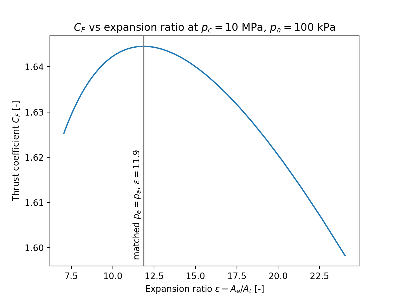
Let us plot the effect of expansion ratio on thrust coefficient:
"""Effect of expansion ratio on thrust coefficient."""
import numpy as np
from matplotlib import pyplot as plt
from proptools import nozzle

p_c = 10e6    # Chamber pressure [units: pascal]
p_a = 100e3    # Ambient pressure [units: pascal]
gamma = 1.2    # Exhaust heat capacity ratio [units: dimensionless]
p_e = np.linspace(0.4 * p_a, 2 * p_a)    # Exit pressure [units: pascal]

# Compute the expansion ratio and thrust coefficient for each p_e
exp_ratio = nozzle.er_from_p(p_c, p_e, gamma)
C_F = nozzle.thrust_coef(p_c, p_e, gamma, p_a=p_a, er=exp_ratio)

# Compute the matched (p_e = p_a) expansion ratio
exp_ratio_matched = nozzle.er_from_p(p_c, p_a, gamma)

plt.plot(exp_ratio, C_F)
plt.axvline(x=exp_ratio_matched, color='grey')
plt.annotate('matched $p_e = p_a$, $\epsilon = {:.1f}$'.format(exp_ratio_matched),
            xy=(exp_ratio_matched - 0.7, 1.62),
            xytext=(exp_ratio_matched - 0.7, 1.62),
            color='black',
            fontsize=10,
            rotation=90
            )
plt.xlabel('Expansion ratio $\\epsilon = A_e / A_t$ [-]')
plt.ylabel('Thrust coefficient $C_F$ [-]')
plt.title('$C_F$ vs expansion ratio at $p_c = {:.0f}$ MPa, $p_a = {:.0f}$ kPa'.format(
    p_c *1e-6, p_a * 1e-3))
plt.show()
(Source code, png, hires.png, pdf)
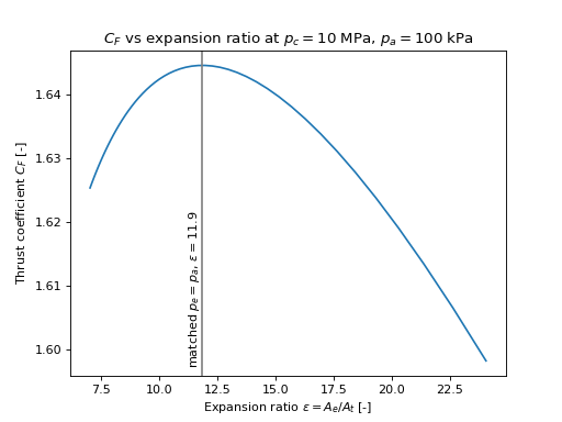
The thrust coefficient is maximized at the matched expansion condition, where \(p_e = p_a\). Therefore, nozzle designers select the expansion ratio based on the ambient pressure which the engine is expected to operate in. Small expansion ratios are used for space launch boosters or tactical missiles, which operate at low altitudes (high ambient pressure). Large expansion ratios are used for second stage or orbital maneuvering engines, which operate in the vacuum of space.
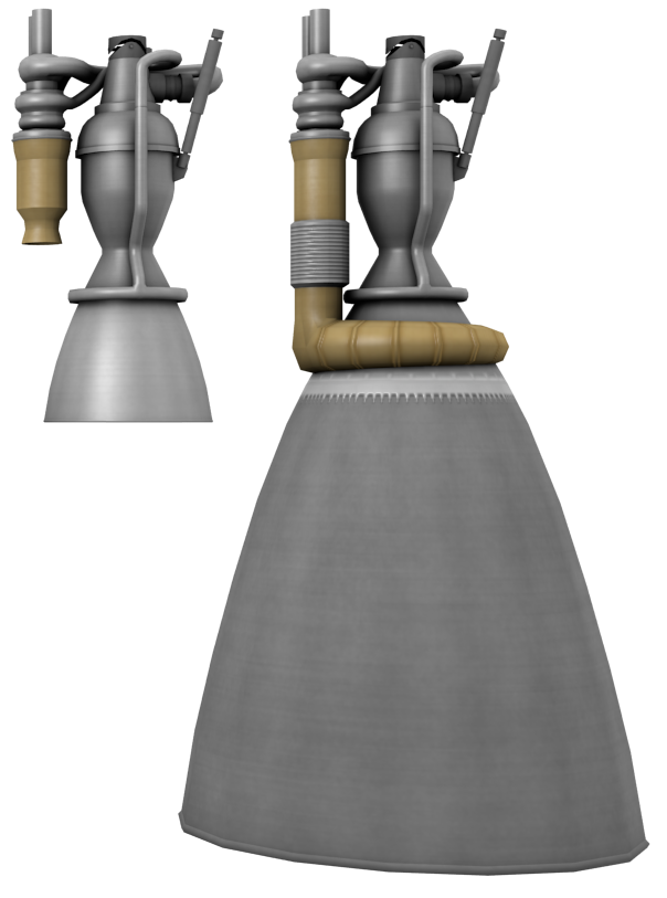
This illustration shows two variants of an engine family, one designed for a first stage booster (left) and the other for a second stage (right). The first stage (e.g. sea level) engine has a smaller expansion ratio than the second stage (e.g. vacuum) engine. Image credit: shadowmage.
The following plot shows \(C_F\) vs altitude for our example engine with two different nozzles: a small nozzle suited to a first stage application (blue curve) and a large nozzle for a second stage (orange curve). Compare these curves to the performance of a hypothetical matched nozzle, which expands to \(p_e = p_a\) at every altitude. The fixed-expansion nozzles perform well at their design altitude, but have lower \(C_F\) than a matched nozzle at all other altitudes.
"""Plot C_F vs altitude."""
import numpy as np
from matplotlib import pyplot as plt
import skaero.atmosphere.coesa as atmo
from proptools import nozzle

p_c = 10e6   # Chamber pressure [units: pascal]
gamma = 1.2    # Exhaust heat capacity ratio [units: dimensionless]
p_e_1 = 100e3    # Nozzle exit pressure, 1st stage [units: pascal]
exp_ratio_1 = nozzle.er_from_p(p_c, p_e_1, gamma)    # Nozzle expansion ratio [units: dimensionless]
p_e_2 = 15e3    # Nozzle exit pressure, 2nd stage [units: pascal]
exp_ratio_2 = nozzle.er_from_p(p_c, p_e_2, gamma)    # Nozzle expansion ratio [units: dimensionless]

alt = np.linspace(0, 84e3)    # Altitude [units: meter]
p_a = atmo.pressure(alt)    # Ambient pressure [units: pascal]

# Compute the thrust coeffieicient of the fixed-area nozzle, 1st stage [units: dimensionless]
C_F_fixed_1 = nozzle.thrust_coef(p_c, p_e_1, gamma, p_a=p_a, er=exp_ratio_1)

# Compute the thrust coeffieicient of the fixed-area nozzle, 2nd stage [units: dimensionless]
C_F_fixed_2 = nozzle.thrust_coef(p_c, p_e_2, gamma, p_a=p_a, er=exp_ratio_2)

# Compute the thrust coeffieicient of a variable-area matched nozzle [units: dimensionless]
C_F_matched = nozzle.thrust_coef(p_c, p_a, gamma)

plt.plot(alt * 1e-3, C_F_fixed_1, label='1st stage $\\epsilon_1 = {:.1f}$'.format(exp_ratio_1))
plt.plot(alt[0.4 * p_a < p_e_2] * 1e-3, C_F_fixed_2[0.4 * p_a < p_e_2],
    label='2nd stage $\\epsilon_2 = {:.1f}$'.format(exp_ratio_2))
plt.plot(alt * 1e-3, C_F_matched, label='matched', color='grey', linestyle=':')
plt.xlabel('Altitude [km]')
plt.ylabel('Thrust coefficient $C_F$ [-]')
plt.title('Effect of altitude on nozzle performance')
plt.legend()
plt.show()
Characteristic velocity
We can define another performance parameter which captures the effects of the combustion gas which is supplied to the nozzle. This is the characteristic velocity, \(c^*\):
For an ideal rocket, the characteristic velocity is:
The characteristic velocity depends only on the exhaust properties (\(\gamma, R\)) and the combustion temperature. It is therefore a figure of merit for the combustion process and propellants. \(c^*\) is independent of the nozzle expansion process.
The ideal \(c^*\) of the example engine is:
"""Ideal characteristic velocity."""
from proptools import nozzle

gamma = 1.2    # Exhaust heat capacity ratio [units: dimensionless]
m_molar = 20e-3    # Exhaust molar mass [units: kilogram mole**1]
T_c = 3000.    # Chamber temperature [units: kelvin]

# Compute the characteristic velocity [units: meter second**-1]
c_star = nozzle.c_star(gamma, m_molar, T_c)

print 'Ideal characteristic velocity = {:.0f} m s**-1'.format(c_star)
Ideal characteristic velocity = 1722 m s**-1
Specific Impulse
Finally, we arrive at specific impulse, the most important performance parameter of a rocket engine. The specific impulse is the ratio of thrust to the rate of propellant consumption:
For historical reasons, specific impulse is normalized by the constant \(g_0 =\) 9.807 m s -2 , and has units of seconds. For an ideal rocket at matched exit pressure, \(I_{sp} = v_2 / g_0\).
The specific impulse measures the “fuel efficiency” of a rocket engine. The specific impulse and propellant mass fraction together determine the delta-v capability of a rocket.
Specific impulse is the product of the thrust coefficient and the characteristic velocity. The overall efficiency of the engine (\(I_{sp}\)) depends on both the combustion gas (\(c^*\)) and the efficiency of the nozzle expansion process (\(C_F\)).
| [RPE] |
|